

This section covers technical details of software, hardware and operation.
Software
The software for this project comprises over 8,000 lines of code written in Python 3.7, not including test programs and third party libraries such as Redboard and Adafruit etc.
Basic concepts
There are two levels of control: simulator level where a supervisor determines what configuration will be run and when, and operator level where a grid operator interacts directly with the running simulator via a physical control panel. The supervisor rôle is taken by a trained member of staff and the operator rôle by a participating visitor. The diagram below shows the main simulation loop which controls the operation of the models.
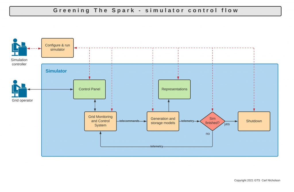
The prime function of the main simulation loop is to provide the timing needed for loop iteration and synchronisation of the models. Every model has code for initialisation and looping. Other functions include storing simulation information for further analysis and compiling a simulation report or displaying the results of a game.
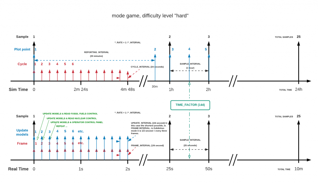
The simulation runs in simulation time but the actual software runs in real time. The relationships between quantities measured in these two time frames are illustrated in the diagram above. The rate at which simulation time runs faster than real time is called the time factor, like fast forward on a video player. For example, a time factor of 144 allows a 24 hour simulation to complete in 10 minutes.
Due to hardware limitations* the fastest loop iteration speed is 6 Hz (real time) which is plenty for this project where pinpoint precision isn’t needed. Integrations of power to energy are linear but, as the changes are small and generally cyclical over the periods concerned, errors are small and not cumulative.
*The time taken to process analogue inputs is ~130ms so, together with updating the control panel displays, they are scheduled into three separate iterations: update displays, input 1, input 2. This happens twice a second making a total of 6 iterations per second, or 6 Hz. If the simulator gets behind, it can catch up by increasing the delta sim time between iterations. This is especially necessary after a game has been played, because exhibit mode runs in real time, but loses up to 10 minutes when a game is played.
Control System and Models
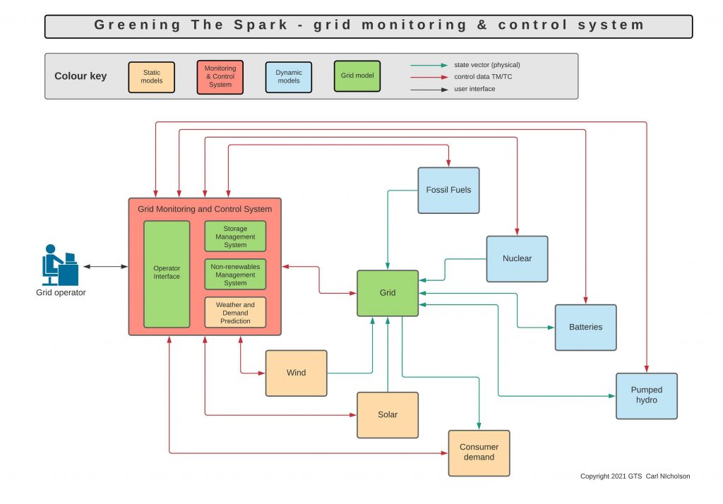
Grid controller operation is based on a spacecraft monitoring and control system (MCS) model which reads telemetry (TM) from the various subsystems, takes input from the grid controller, interprets the control laws and then sends telecommands (TCs) back to those subsystems. This process repeats in a continuous loop until the simulation is finished. The MCS also contains a Storage Management System (SMS) which determines how energy is to be stored and retrieved in order to maintain a balanced grid. There is also a non-renewables management system (NMS) for autonomous control of fossil fuels and nuclear. In autonomous mode these sources are controlled without operator input. In the museum version there is a semi-autonomous mode where the NMS is in control by default and manual control is triggered by touching one of the controls. Autonomous control resumes when there has been no user input for a predetermined amount of time.
Static models run scenarios based on predefined weather and consumer demand patterns. Weather models include wind speed, solar intensity and temperature (although temperature isn’t used in the museum version – it is planned as an input to the consumer demand model). A pattern is defined as a uniform set of samples over a timeline. The value at any given moment is linearly interpolated between its enclosing samples. The samples in a timeline file represent a baseline from which actual and forecast timelines are calculated. These derived timelines are calculated from the baseline by addition of random Fourier components at DC, half wave, full wave and sample frequencies whose coefficients are a function of the difficulty level*. Forecasts can be either literal or differential, indicating what change is expected over the next sample interval.
*Difficulty level is a game type parameter affecting the volatility and predictability of timelines, response times of the non-renewables and the scale of storage elements, the end result being to make controlling the grid less or more challenging.
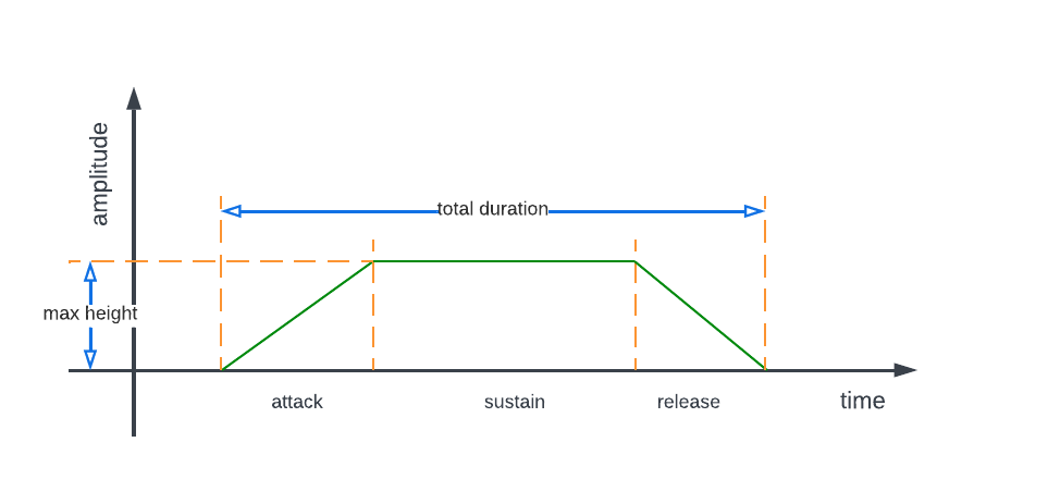
In addition to the timeline based weather models, and to add an extra degree of realism, short term variability is introduced in the form of gusts of wind, clouds and surges in consumer demand, collectively known as bursts. These are like randomly generated midi notes with start time, attack, sustain and release parameters being randomly generated to create bursts lasting in the order of tens of seconds. This feature is only run in exhibit mode, as games run much faster than real time and bursts wouldn’t get noticed.
Dynamic models include generation by fossil fuels and nuclear facilities which are controlled by the grid operator via the MCS control panel or autonomously by an NMS, and storage devices which respond to telecommands from an SMS.
Autonomous control (by the NMS) of the dynamic models can follow various strategies depending on priorities and sophistication. A simple model follows the difference between renewables and demand and allocates power proportional to generators’ capability. A better model takes storage into account. Other strategies include minimising cost or carbon dioxide emissions. or a compromise between the two.
Storage models are defined by two parameters: maximum power and capacity. Power is the rate at which a storage device can charge or discharge and capacity is the total energy a device can store. The amount of energy stored as a fraction of the capacity is called the level, so a half-full battery has a level of 0.5, or 50% (the same as a half-empty one).
Losses in the charge / discharge cycles for batteries and pumped hydro are modelled with a configurable parameter efficiency set to a default of 80%, typical of industrial installations. Reduction in capacity over time, differences in maximum charge and discharge rates, and delays or limits to changing the charge and discharge rates are not modelled.
There is always a discrepancy between generation and demand. The Storage Management System (SMS)* manages the storage devices with a view to meeting demand (no shortfall) and avoiding waste (no surplus).
*Storage devices are ranked by level. When excess power is generated, the device with the lowest level is charged first at up to its maximum charge rate unless full. If more power needs to be sinked then the next device up in the level hierarchy is charged in the same way. This continues with the remaining devices as necessary. If the storage devices cannot sink all the excess power, then the MCS registers a grid status of surplus and the grid surplus LED is illuminated. Discharging works the other way round, where the device with the highest level is discharged first etc. If the storage devices cannot make up all the deficit and more power is still required by the grid, then the MCS registers a grid status of shortfall and the grid shortfall LED is illuminated. In all other cases the grid status is nominal.
Operation
Operation is divided into two rôles: staff, who work via the staff control panel, and visitors, who use the visitor and operator control panels (see picture below). A typical startup, operation and shutdown sequence is as follows:
Staff:
- Switch on the installation.
- Stop/start lamp illuminates when RPi has booted up and started the main program.
- Hardware Test mode is entered and all hardware components exercised.
- If everything is ok, the simulator goes into autonomous exhibit mode, running in real time with the clock showing the actual time of day. The play button and auto LEDs are illuminated ready for action. An ambient soundscape provides convincing background sounds you might expect in a national grid control centre.
Visitor:
- Trigger motion sensor by walking up to the exhibit. This enables the representations: sun lamp and wind turbines become operational. The audio virtual guides spring into action and the visitor is welcomed and given an explanation of everything they see in front of them.
- Inspect the exhibit, browse information, instructions etc.
- Touch one of the knobs and take control of the non-renewables (fossil fuels and nuclear). More feedback from the audio guides.
- Press play button. Game number is displayed.
- Choose difficulty level.
- Press start button. Audio messages explain how the game is played (or abandoned after a fixed period of inactivity).
- Play the game. Game starts after the audio explanation has finished and an energising game soundscape is then played, culminating in a loud “Countdown” style clock ticking as the game draws to a close.
- Results are displayed by the colours of the three sparks on the visitor control panel and a full verbal explanation is given. Results are also sent to the online database and can be viewed by entering the game number (for more information see below in section “Reporting”).
- Exhibit returns to autonomous exhibit mode.
- Representations de-activate until next visitors trigger the motion sensor again. (This is an energy and wear and tear saving feature for the lamp and model wind turbines.)
Staff:
- Press the stop/start button.
- Switch off the installation.

Visitor Centre
The visitor centre is an information resource available online and on site on the touch panel part of the display. The information content can be browsed from the Visitor Centre entry in the main menu.
Audio
Adding audio has given a whole new dimension to GTS in terms of ambience and narrative, bringing the installation alive. Sound effects are played as a background soundscape, an indication of something happening or a warning. Three characters inform (and entertain) staff and visitors with synthesised speech. Examples below:
This has been made possible by developing / exploiting these key components:
- MP3 player that works(!)
- Python parallel processing & command line interface
- Speech synthesis & sound effects
- Sound processing
Finding an MP3 player that worked proved to be problematical as various Python players (playsound, pygame) simply refused to work on the target Raspberry Pi. Finally I had to use omxplayer, which is called from Python using the standard OS system command method.
Playing audio files can’t be allowed to interfere with the operation of the models which mostly run in a continuous loop, so Python’s capability of creating and running independent parallel processes was used, also not without problems. In test programs audio files would continue playing after the program terminated, resulting in the Python IDE crashing. This has been avoided in the Main Simulation Application (MSA) by the judicious insertion of sleep() intervals (but not in the simulation loop itself).
Audio is normally triggered by the occurrence of an event (as are various other processes). This has resulted in five new utilities being written:
- Transition detector – detects a change of state and responds either immediately or after a specified time delay, during which it is pending. It also allows for locking, which prevents retriggering for a specific time interval (useful for jittery state changes like batteries full / not full).
- Scheduler – allows scheduling of events at fixed times or first time and then repeated at fixed or random intervals
- Audio file queue handler – to avoid clashes when simultaneous events trigger different audio responses
- Toggler – simply changes a binary state
- Interlock. Allows coordination of activities when a resource is used by more than one “client”.
A custom playlist handler was written to enable audio to be played easily from anywhere in the GTS code. It has the following features:
- Plays playlists and single audio files
- Can play sequentially, where the program stops until the list has finished playing, queued, where files are put in a queue and played in parallel with the program thread or in ambient mode, when audio files can play in parallel without being queued
- Queue handling consists of two parts: adding a file to the queue and servicing the queue to play the next one when it comes due
- Multi-version playlists can be called with a specific version, cyclic or random. This is to allow a variation in audio responses to common events.
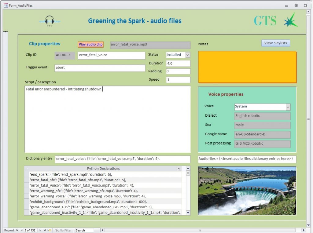
Events, voices, sound effects, voice messages (text & parameters), audio files and playlists are all documented in the GTS Audio database which also generates declarations for inclusion in the audio data Python module.
Speech synthesis is possible thanks to Google Cloud Services Text to Speech and sound effects are largely courtesy of Freesound.
Post processing of the audio files is done in Ableton Live where necessary (eg. robotic GTS system voice) with the final editing being done in Goldwave.
Reporting
Simulation Report
Sparks are awarded on overall performance* in three “E” categories: Efficiency, Eco-friendliness and Economy where :
- Red spark is the worst
- Green spark is the best
- Blue spark is in between
Sparks are calculated as a weighted average of relevant points and converted to a colour.
A report is generated for each game played, accessible in an online database by entering a unique game number. A csv file is also created for further processing / archiving.
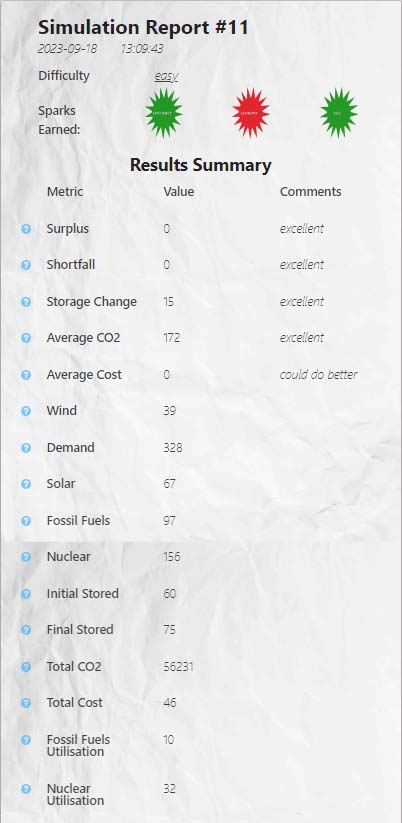
These reports contain the following information:
Summary data, comprising date and time, total energy generated, used and stored, utilisation of various generators, total and average of costs incurred and CO2 produced. Comments and scores are attached to quantities which indicate how well a grid operator has performed; they are generally calculated by comparing to a best or worst case and assigning points accordingly*. Ranges are defined to map comments to scores.
*Shortfall and surplus points are are calculated as a function of that quantity divided by total demand. If the total demand is zero, then the shortfall can only be zero. However, surplus can still be positive resulting in division by zero which computers don’t like (or exceedingly large numbers when demand is very small). The function used is a scaled arctan (tan-1 for mathematicians), which happily deals with numbers from nought to infinity, with a trap for division by zero (which computers do not).
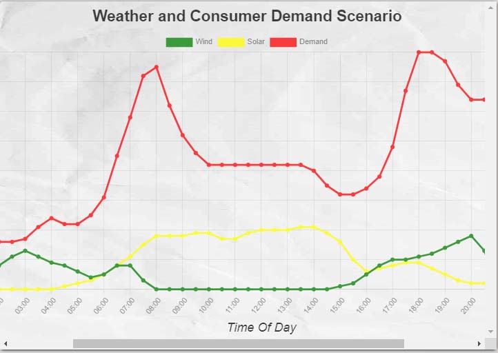
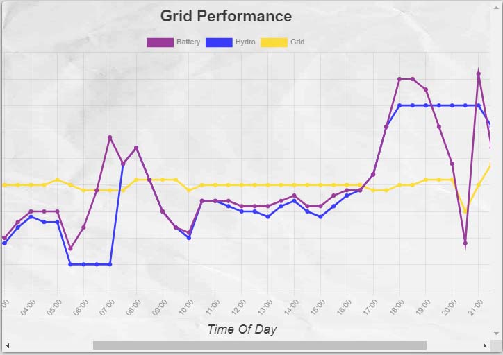
Timelines are included in the simulation report as three sets of data plotted against time over a 24 hour period. These are:
- Inputs. These are the given scenarios: wind speed, solar intensity and consumer demand
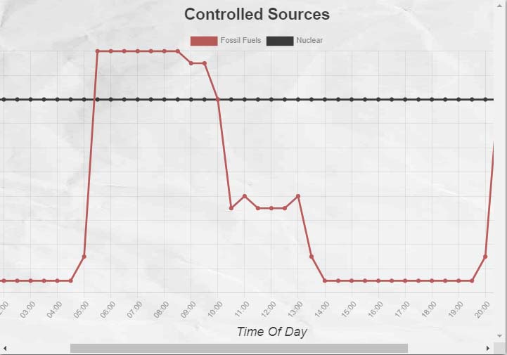
- Controls. These are the two generators the visitor has control over via the control panel knobs: Fossil Fuels and Nuclear
- Outputs. These are the consequences of the visitors’ actions: how the power generated stacks up against demand (surplus, nominal and shortfall) and the resulting state of the storage devices (from full to empty).
Other Reporting
Of course the Simulation Report is the only report most people will ever see (or care about), but it is just the tip of the iceberg. There are three other kinds of report that generate huge amounts of data for general diagnostics and analysis:
- Configuration log files containing a full account of all the parameters used to define the models and operation of the GTS for a given day
- Logbook log files. These are a record of all system level events reported in a day’s sessions
- Plot files. These are the timelines generated in a day’s sessions
- A copy of the games results (identical to those posted online for Simulation Reports).
Timeline reporting requirements vary according to intended use; for example a plot file might require samples every 5 seconds, whereas a simulation report might need them only every 30 minutes. The models run at 6Hz, so potentially the maximum sample rate is 6Hz, which would generate far too much data if it was all recorded. Taking regular samples at less than that rate does not represent what is happening in between samples, so a simple resampling algorithm has been written in which a group of samples is represented by their average value. This preserves their aggregate sum; for example it allows the total energy to be calculated from power samples, no matter what the sampling rate. [Accurate delta function resampling, with an appropriate low pass filter and subsequent sinc function reconstruction are beyond the needs of this project.]
Hardware
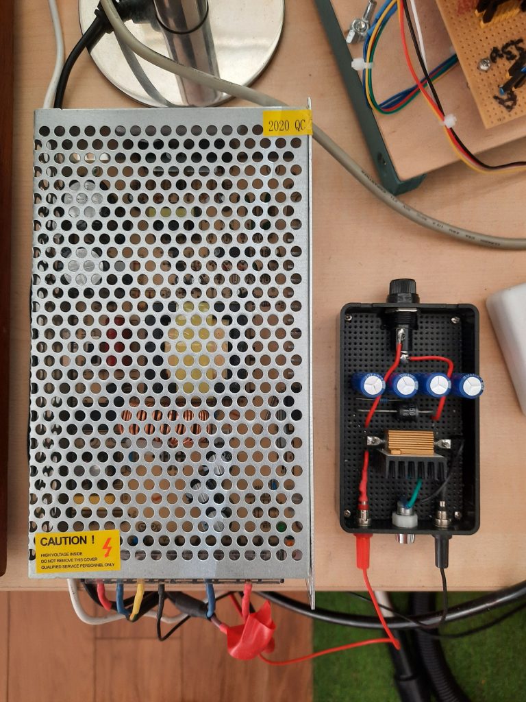
Power
The power comes from a 12V 20A switched mode PSU with a custom “glitch-buster” ultra-capacitor (4*10F@3V in series) storage device which can supply power for up to a minute in the event of power failure.
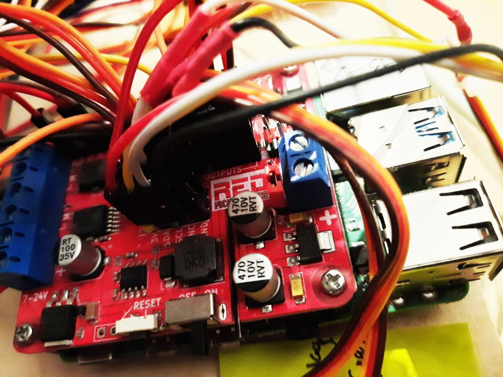
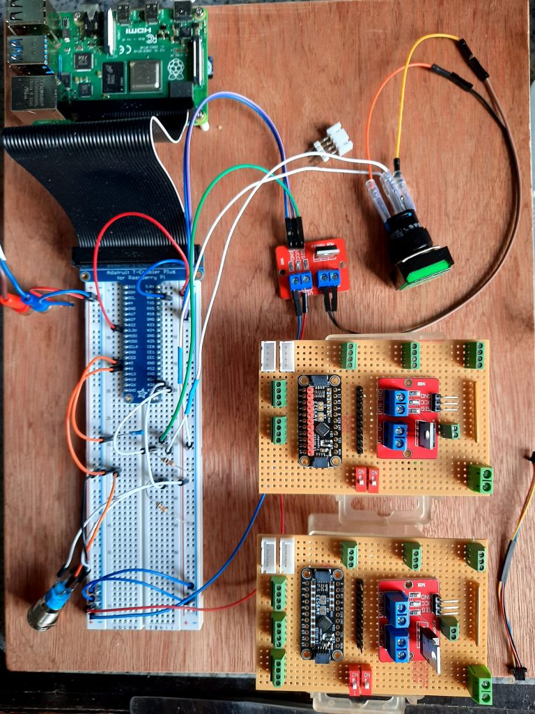
Raspberry Pi
The Raspberry Pi’s are model 4Bs with 8GB ram and 32GB flash cards. The GTS one is fitted with a Red Robotics Redboard+.
This is the Raspberry Pi development area with an Adafruit T-Cobbler Plus connected to a breadboard.
Operator Control Panel
The control panel comprises:
- The main panel with artwork created in Lucid Chart and printed on aluminium. This was machined to fit the components and mounted on a wooden frame.
- A numeric header was added later, using a wooden panel with artwork printed on glossy photo paper and glued to the panel, for four displays indicating either time, mains frequency, CO2 and cost or power generated by each source.
- A switch to control which set of numbers is displayed on the numeric header
- Two renewables generator panels (wind & solar), with gauges displaying actual power being generated and relevant weather forecasts (wind & sun)
- Two non-renewables panels (fossil fuels & nuclear), with knobs for controlling the power and gauges for displaying how much power is being generated
- A consumer demand panel with gauges displaying how much power is being used and a demand forecast
- A status panel with bar LEDs showing storage status (batteries and pumped hydro) and single LEDs showing overall grid status (shortfall, nominal, surplus)
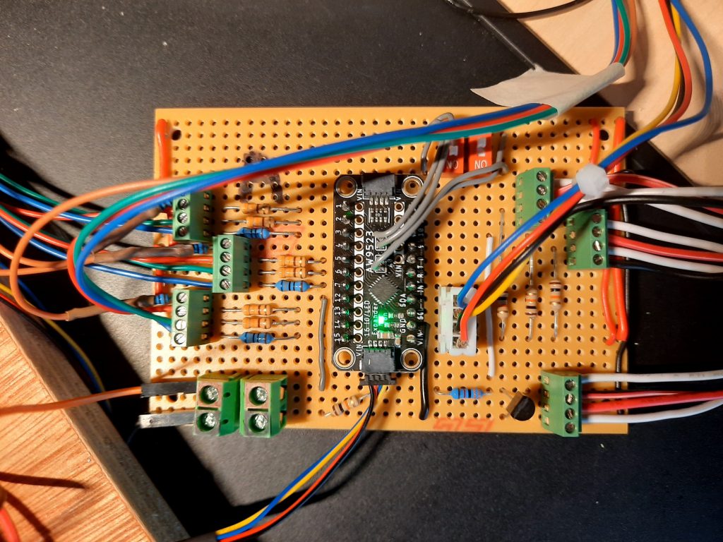
All hardware is interfaced to the RPi via the Redboard+ hat. The various hardware types and connections are as follows:
- Four numeric displays are Adafruit 4 digit 7 segment LEDs, connected via an I2C bus.
- Numeric header switch is connected to a spare input on the batteries expander board (see below).
- Eight gauges are stepper motors connected to the stepper motor ports.
- Two potentiometers (the control knobs) are connected to the ADC ports.
- Three grid status LEDs are connected via a discrete NOR logic board requiring only two GPIO pins.
- Two storage status 10 bar LED arrays are connected to an Adafruit GPIO expander on the I2C bus.

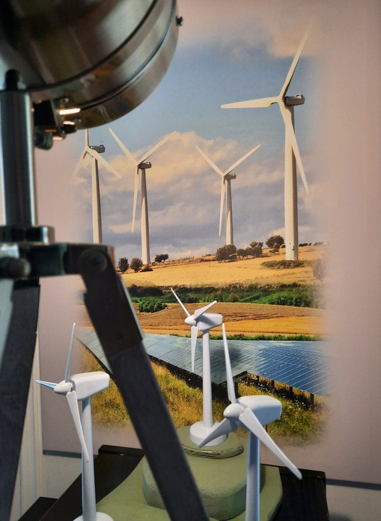
Representations
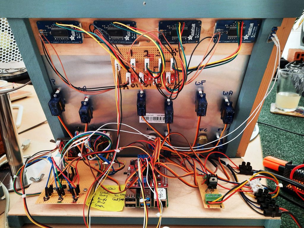
There are representations of a wind farm with three model wind turbines and a sun lamp in front of a mural depicting actual wind and solar farms. These are controlled via the Redboard+ PWM motor ports, the turbines directly and the sun lamp via a custom Darlington pair driver circuit (just visible in the bottom right of the rear view picture) for extra ‘oomph, getting its power directly from the PSU.
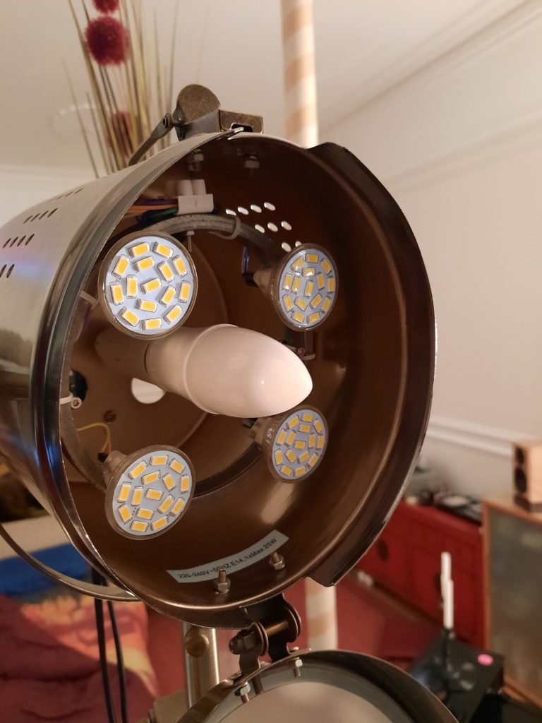
The sunlamp has four high power 12V LED arrays powered by GTS and it also has a mains bulb so it can function as a normal room light when GTS is off.
Calibration
The servos which drive the gauges need calibrating for both position and scale. There is a calibration program which uses the two power input control knobs (fossil fuel = coarse and nuclear = fine) to generate a voltage to control servo positions. Each servo is calibrated in turn for zero and full scale deflection, with the position values entered into the calibration file. Two modes of operation are possible, set by a simulation parameter at run time : full scale or proportional (standardised). Full scale uses the gauge FSD as the maximum power for that generator and standardised uses the FSD for the maximum power of the demand. Each gauge can show up to 110% FSD, limited by software to protect the servos from damage.
Power control knobs are calibrated for both position and scale. Each knob is calibrated in turn for zero and full scale deflection, with the measured voltages entered into the calibration file.
Representations. The solar lamp needs no calibration measurement as such: zero is off and 100% PWM is fully on; scaling is provided in the calibration file to match sun intensity to lamp brightness, using the maximum sun intensity anywhere on earth as a guide. The wind turbines, however, are a bit more complicated.
With wind turbine models it is necessary to match up the stall and maximum safe speeds of the physical models with realistic stall and maximum safe wind speeds of a real turbine. Hysteresis complicates matters as the actual stall speed is different depending on whether it is slowing down or speeding up. Using the control knobs as before, calibration software allows the stall speed in both directions to be measured as a PWM % sent to the model. The natural stall speed of the model is then overridden in software so that anything below the stall wind speed is interpreted as zero power and the turbine behaves more or less as expected.* The maximum speed of the model turbines is set so as look realistic and not wear out too quickly.
Ideally, if a turbine is moving then wind power is registered on the grid and conversely, if none is moving, then no power is registered. However, a bit of artistic license can be applied here: if power is registered when no turbine is moving, then we can say it must be from ones on the other side of the hill. Conversely, if no power is registered when turbines are moving, then they may be rotating but not generating, perhaps faulty, undergoing maintenance or just not connected to the grid.
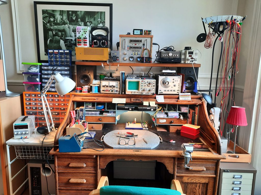
Hardware Central
This is where the chips are fried and other components and boards tested to destruction. Happy days.
List of acronyms
- FSD Full Scale Deflection
- GTS Greening the Spark
- MSA Main Simulation Application
- MCS Monitoring and Control System
- NMS Non-renewables Management System
- PWM Pulse Width Modulation
- SMS Storage Management System
- TC Telecommand
- TM Telemetry
- URN Unique Report Number